Example result

A run on real data from a low-frequency aperture array (EDA2): a 151 MHz observation in XX, crossed by several Starlink satellites.

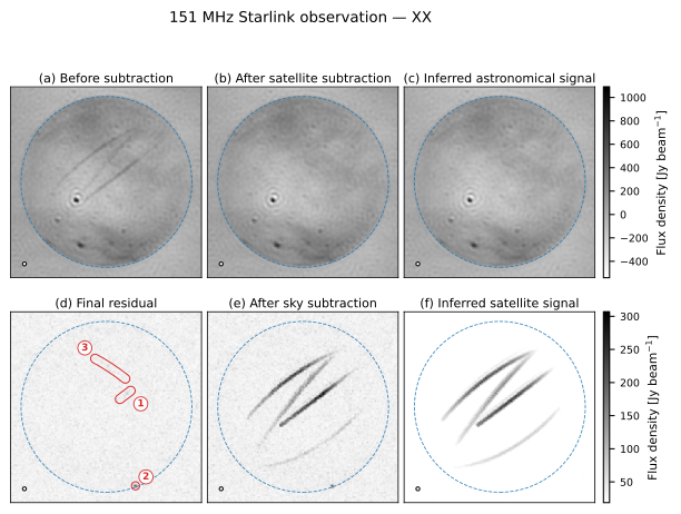
The dashed circle marks the field of view and the small open ellipse at lower left is the synthesised beam. The two rows use different flux scales: the sky spans roughly -400 to 1000 Jy/beam, while the satellite signal is a few hundred Jy/beam.

Reading the panels

The top row follows the subtraction:

• (a) Before subtraction — the satellite trails cross the field, bright enough to dominate it.

• (b) After satellite subtraction — the trails are gone.

• (c) Inferred astronomical signal — the sky component the model fitted, which is what (b) is left showing.

The bottom row runs the same split the other way, which is the more informative check:

• (e) After sky subtraction — remove the sky model instead, and the trails are what remains.

• (f) Inferred satellite signal — the model’s own reconstruction of those trails. That (e) and (f) agree is the point: the split was not simply a smoothing that removed a bright feature, but a model that accounts for it.

• (d) Final residual — what neither component explains. It is noise-like apart from the marked features.

Why the trajectory matters

The satellites are separated from the sky because their trajectories are known. A satellite moves through the field, so its contribution to each visibility carries a fringe rate set by its motion, quite different from the sidereal rate of the sky. TABASCAL models that motion explicitly rather than flagging the affected data, which is what makes it possible to recover the sky underneath a trail rather than discarding it.

This also sets out the method’s main requirement: an orbit good enough that the predicted phase tracks the real one. Orbit sourcing and accuracy are covered in Satellite orbit records.

For the method itself and its validation, see the papers linked from the README.